Anomaly Detection Using Normal Behavior Modeling (NBM) for Predictive and Prescriptive Maintenance

Normal behavior modeling (NBM) is an approach to process, system, and equipment management and maintenance that has been enabled by recent advances in the fields of artificial intelligence (AI) and machine learning (ML). This white paper describes the evolutionary forces that have led to this new capability set, its applications (current and prospective), its benefits, and details of how the technology works. In addition to the explanation of NBM’s operation and implementation, several examples are provided that highlight the benefits of this technology.

Introduction

The primary goal of this white paper is to provide an in-depth introduction to the topic of NBM so that corporate decision-makers will understand its capabilities, requirements, and potential limitations, thus enabling them to make informed decisions about the technology’s applicability to their particular operational challenges. Much has been written about AI in recent years and, in particular, its ability to identify anomalies in the otherwise normal operation of equipment and processes. But there remains an air of mystery about the technology, especially concerning the ways in which specific alerts and notifications are generated and how they should be responded to (if at all). There is, in short, a bit of a ‘black box’ aspect to AI and techniques like NBM, and it is our goal to provide a peek inside that box.

In addition to providing some insight into how NBM works, a further objective of this white paper is to identify specific use cases in which it delivers tremendous business value. NBM is applicable to a wide range of operational fields-–in practice, any in which ‘normal’ operation can be quantified from available data—and we will identify several of them. They include everything from maintaining the reliability of production assets in manufacturing plants and oil & gas facilities to optimizing financial investment decisions and the operation and maintenance activities of aviation and maritime shipping firms.

Modern industrial equipment routinely costs millions of dollars, both to purchase and to operate. The goal of any industrial concern is not only to employ that equipment to maximize production but also to manage ongoing expenses by minimizing routine or unscheduled maintenance and increasing the useful lifetimes of these expensive capital assets. Historically, these goals have been pursued using condition-based monitoring (CBM) solutions or OEM-provided asset management tools incorporating physics-based models. However, in a world where equipment is increasingly more reliable, and failure data is scarce, traditional approaches which rely primarily on it are far less effective than the NBM approaches described here. The goal of NBM is to facilitate the achievement of these goals, i.e., minimizing operational costs while maximizing revenue generation and equipment lifetime, in a more proactive and effective manner. But before diving into the details of how NBM accomplishes these things, it’s worth taking a moment to consider how we have gotten to where we are today in the field of NBM-based anomaly detection.

Evolution of maintenance approaches

As suggested earlier, normal behavior modeling is an analytical technique that can be applied to either an entire end-to-end process or just one particular piece of equipment, say, a hydraulic pump or wind turbine. However, long before the term NBM came into existence—indeed since the invention of the very earliest mechanical devices—equipment and process operators have been tasked with keeping them running for as long and as continuously as possible.

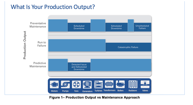
In the earliest days, this meant nothing more sophisticated than repairing a piece of equipment when something failed (run-to-failure approach). If a wheel on your oxcart broke, you either repaired it on the spot or you took it to a wheelwright who fixed it or sold you a new one. This approach is ideal for assets/machines that are very cheap to replace, and the asset failure will not cost catastrophic damage to adjacent assets or harm to human lives.

As time and technology progressed, operators got better at identifying conditions suggesting that a failure was imminent, and they became equally creative at coming up with maintenance actions they could take in advance to prevent an all-out failure. It was the birth of preventive maintenance. With a better understanding of how pieces of the machine would degrade over time, experts would set “expiration dates” for critical pieces of the equipment, and replace it periodically. Note that because expiration dates were set arbitrarily, and based on average life of each component, oftentimes perfectly good parts were replaced adding costs for the new parts, as well as unnecessary downtime to install the parts.

By the time of the industrial revolution in the late 1800s, with the arrival of textile and paper mills, munitions factories, etc., the equipment had become quite complex and frequently temperamental to operate, meaning that factory bosses had to employ experts whose sole purpose was to keep everything running smoothly. Frequently the expertise required to do this job was no more complex than listening to the sounds a machine made, feeling its vibrations, or staying alert to unusual smells. Eventually, though, mechanical gauges arrived on the scene, and industry had its first sensors, a new capability that still plays a critical role to this day. Now, with the ability to monitor quantified measures like temperature, pressure, and flow rate, and to track these measures over time, the possibility emerged of understanding what qualified as ‘normal’ behavior for a piece of equipment and foreseeing when something was beginning to go wrong – it was the early days of predictive maintenance fully powered by human experts using their senses to and intuition to “predict” when a piece of equipment needed maintenance.

Fast forward to the middle of the twentieth century, and operations experts were applying statistical techniques to interpret the growing quantities of data they were collecting (often manually) on their systems. Increasingly advanced mathematical techniques were applied to operational data, culminating in the 1970s and 1980s with the emergence of statistical process control (SPC), a sophisticated ability to identify upper and lower tolerances for a specific performance measure and to automatically identify when a tolerance was exceeded, often an early indication of an incipient problem. There were, though, a couple of important limitations of these techniques. First, the time-series data were typically applied to a single metric, e.g., the pressure of a pump, the temperature of a reactor, etc. The ability to combine numerous values into a single holistic view of system performance was still very much in the future. Further, the threshold alerts provided by SPC systems were frequently indicative of a problem that was already occurring, meaning it was quite late in the game to do anything proactive about it.

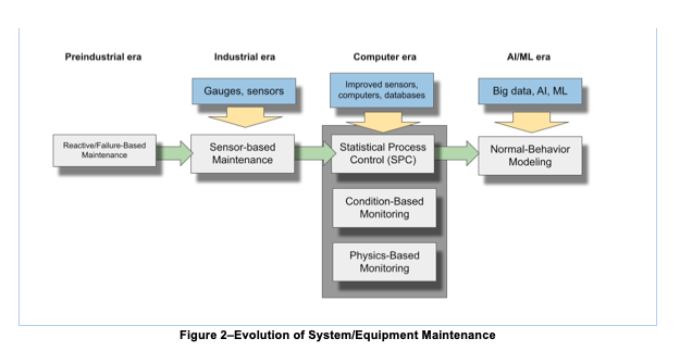
Around this same time, the notions of condition-based and physics-based performance modeling began to take precedence. In the former case, operators conducted continuous monitoring of numerous sensor outputs, based either on their own knowledge of system operations or on guidelines provided by original equipment manufacturers (OEMs) of these systems. By evaluating equipment performance in real-time, operators became aware of problems, though typically with little or no advance notice, rendering repairs very much an after-the-fact situation.

Physics-based models, on the other hand, relied on subject matter experts to simulate/model the operation of a system or piece of equipment by defining it with a series of static mathematical equations. These equation sets could do a good job of defining a system’s operation under predictable conditions, but broke down quickly in dynamic conditions, whether those dynamic conditions were internal to the system or exogenous (such as weather events, etc.). Despite the limitations of these methodologies, many system operators today still maintain their equipment using some combination of physics- or condition-based maintenance approaches.

With the turn of the 21st century and the arrival of ‘big data,’ high-bandwidth data transmission, and petaflop computing capabilities, a new universe of possibility came into being. Operators had understood for a long time by now that a system’s overall performance-–its ability to do its job—depended not only on the correct values of individual performance measures right now but rather on the collective achievement of many such measures working in concert over extended time periods. Additionally, with machines becoming ever more reliable, failure data is becoming scarce, thus compromising the efficacy of physics-based models, which relies heavily on failure data to feed and mature models prior to deployment. And it is this need that normal behavior modeling satisfies with increasingly great precision.

Data cleaning and filtering

As with any data-driven analytical exercise, the quality of data provided to the NBM model will go a long way toward maximizing the quality of output results (in this case, the veracity of alerts).

Thus the removal of noise from the input data becomes a crucial step when adopting NBM. This could be spurious or out-of-range data or entirely missing data, the latter of which is dealt with by interpolation or inference based on other related data points.

It is a useful first step in any NBM development process to decide on the frequency and granularity of the data that will be used. While it will generally be true that more is better, there will be points beyond which processing times become cumbersome and the value of even more data will begin to result in diminishing returns. Thus, because there exist sensors that provide output data every second and others that provide a reading once each hour, careful consideration should be given to the input data frequency required vs. the timeliness of outputs that will be needed. A commonly employed test of these requirements is to create and run an initial NBM model on a large historical dataset during which known failures occurred, to gauge the extent to which the model can predict those failures post facto. This is not only an excellent tuning exercise prior to model development, it also goes a long way toward creating organizational comfort with the entire modeling process.

Deep learning and neural networks

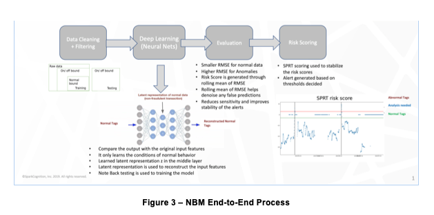
Central to the concept of normal behavior modeling is an algorithm known as an encoder, a high-level diagram of which is shown in Figure 4. The encoder’s input layer ingests a continuous stream of quantitative input data from equipment sensors (temperature, pressure, etc., shown as Xn in the figure) over time – for example once each minute. This data is then fed to a ‘hidden’ or ‘latent’ layer (of which there are typically several) where it gets compressed, i.e., reduced in dimensionality (fewer nodes than in the input or output layers). Numerical weights (a value between 0 and 1) are then applied to each node, with the goal of eventually reproducing the input values at the output layer – this process is typically known as principal component analysis or PCA.

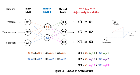
Achieving this outcome typically requires many thousands of iterations, with the weights tweaked slightly with each iteration in response to measured differences between the input and resulting output layers. When the outputs (X’n in the diagram) have finally achieved parity (or as close to it as possible) with the original inputs (Xn) the model is said to have ‘learned’ the normal state necessary to deliver subsequent actionable alerts.

The important aspect of this learning methodology is the reduced number of nodes contained in the hidden layers versus the number of input variables. This is required in order for the model to learn. If the number of hidden layer nodes was equal to the number of input variables (and output results), then the model could simply “cheat” by applying a weight of 1 to every input and instantly recreating the desired output while having learned nothing at all about the system or its operation.

Once the weights have all been accurately assigned and the outputs have been matched as best as is possible to the inputs, the output section of the encoder (the decoder) serves no further purpose until the next iteration of model training and is typically discarded. Having been successfully weighted (i.e., learned the system’s normal state), the NBM model is now ready to evaluate new input data and draw conclusions about its adherence to the normality derived from the model.

Another important element of this modeling process is the notion of output vectors. This concept is demonstrated on the right side of Figure 4. Once model training has been completed, the model is said to have successfully extracted all the ‘features’ from the input training data set. Each of these features is represented by a unique vector comprising as many dimensions as there are unique data inputs (aka ‘tags’) in the input data set. The vector represents a point in multi-dimensional mathematical space that coincides with the weighted combination of all input data elements. It is a critical element of how the model is able to draw its out-of-normal conclusions from the full set of iterating variables rather than from a single variable. In this example, there are only three variables shown, but in fact, each of these vectors contains as many unique dimensions and weights as there are variables in the input data stream, typically dozens, hundreds, or even thousands.

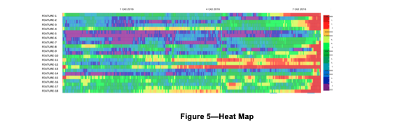
Once vectors are generated, their results are typically displayed on a heat map, as shown in Figure 5. The heat map simply aggregates the degree to which each feature is in or out of tolerance over a period of time (the horizontal axis), with red areas indicating the most out-of-tolerance and green the most in-tolerance. By reordering the feature rows of the heat map to show those with the greatest amount of red (out-of-tolerance) at the top, a snapshot is displayed of the system’s status over the selected period of time.

Evaluation, scoring and alerts

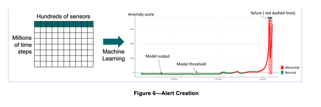
As mentioned in the introduction, one of the key benefits of the NBM approach is that it reduces all of the many thousands of individual time-series data points to a single metric that can be acted upon. This single point is known as a risk score. The risk or anomaly score is the statistical summarization of the extent to which each of the feature vector values deviates from the mean value for that feature (Figure 6).

Determining whether or not maintenance action should be taken based on the anomaly score is a function of how sensitive we want the output to be. In the most basic version of this technique, we would simply assign a threshold value for each anomaly score and declare an alert anytime this value is reached. In reality, this simplistic approach is likely to make the model overly sensitive and generate more false positives (i.e., an alert to a condition that is, in fact, within tolerance and should not be acted upon) than we want.

Instead, it makes sense to decide in advance upon a statistical band of upper and lower bounds derived from experientially determined standard deviations. Thus, it is only when the anomaly score exceeds the upper bound of the band that we will declare the system to be out-of-normal and generate an alert. Limiting alert generation in this way is referred to as utilizing a sequential probability ratio test (SPRT).

Retraining and evolving normals

NBM systems, like all systems, evolve over time. And this evolution takes many forms. Equipment ages, maintenance occurs, tolerances change, desired outputs change, and externalities like availability of time, people, money, and regulations change. As a consequence, our sense of what is ‘normal’ for our complex system is highly likely to change and our modeling approach needs the flexibility to adapt as circumstances evolve. Fortunately, NBM is uniquely well-positioned to respond to these inexorable changes, far more so than the CBM, SPC, and other methodologies discussed earlier.

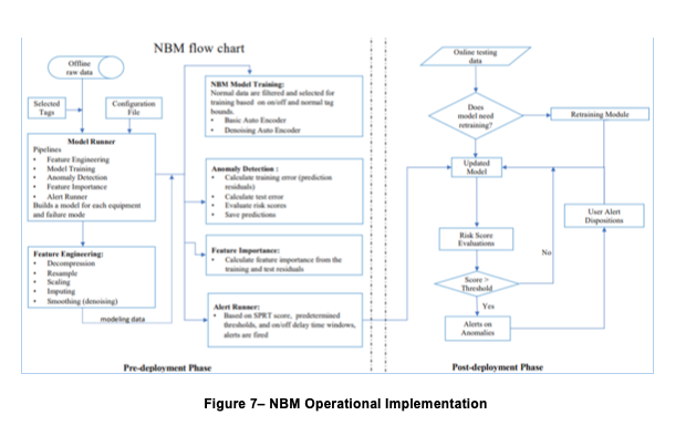
The most straightforward way in which NBM enables this flexibility is simply by retraining it from time to time (monthly is a common choice) to reflect the latest reality. This process occurs in the same manner as initial training, except that in subsequent iterations, results will be improved due to the availability of larger and more comprehensive data sets. In the parlance of our original description, it’s important to build into the ongoing operation of the NBM process the maximizing of the congruence between the model’s inputs and its outputs. The flowchart in Figure 7 shows the way in which initial model creation flows seamlessly into a routine post-deployment phase.

Explainability

There is another extremely important element to consider when making decisions about NBM implementation, and that is the notion of explainability. One of the biggest criticisms that AI receives, in general, is the idea that users are asked simply to trust the system’s outputs without understanding how they were derived. It is thus incumbent on NBM modelers to understand the ways in which the model provides a measure of explainability. In short, it derives from the hidden/latent layer described earlier and, in particular, the role it plays in feature extraction. Inasmuch as a given alert recommendation will likely derive from the anomalous values of numerous data points, close examination of the weights derived by the model and the causal indicators provided by tools like heat maps can go a long way toward explaining the model’s recommendations.

Human-in-the-loop and knowledge management

When diving into the details of AI-enabled NBM model creation and utilization, it’s easy to lose sight of one of the most important resources underlying the entire predictive maintenance process, i.e., the experience and expertise of technical staff members. But they play key roles in making NBM development and use a successful undertaking, including identification of failure modes, establishing functional alert thresholds, and determining when model retraining should be undertaken, to name but a few. At the end of the day, there is simply no replacement for specialized domain expertise, regardless of how much automation a company implements.

Use cases

As previously described, the principal purpose of NBM is to define the normal state of a complex system and to then proactively identify and flag instances in which that system is operating outside of normal. Ideally, such identification and flagging will occur with sufficient advance warning to allow maintenance or repair actions to take place that will forestall an outright system failure and all of the revenue loss, repair costs, and safety compromises that typically come with such failures.There are many examples of complex systems to which NBM techniques can be applied, some of which are physical, others of which are more process-oriented.

Production equipment on oil platforms—Failure can mean millions in lost revenue as well as safety risks and environmental catastrophes. By modeling equipment temperatures, pressures, and rotation and flow rates, incipient problems can be identified early, saving upstream operators millions of dollars and significant regulatory exposure.
Manufacturing plants—Out-of-normal operations in manufacturing plants can result in safety hazards, environmental violations, and inferior quality in the products being produced. Proactive identification of process and equipment problems can help to ensure profitable operations in what are frequently low-margin businesses.
Commercial and military aviation—Jet engines and other complex airborne hardware are routinely subject to enormous operational stresses, and small problems can quickly cascade into expensive and dangerous situations, risking lives as well as the possible loss of immense capital investments.
Financial investments—The normal ebb and flow of global equity and debt markets occasionally undergo upsets that can produce short-lived investment opportunities or risks that must be quickly and actively mitigated. In an industry characterized by millisecond transaction speeds, knowing about these threats and opportunities before the competition can be the difference between success and failure.

Summary and conclusions

Normal behavior modeling is the state of the art in predictive maintenance of complex systems and equipment. It simultaneously automates the complicated process of manual data analysis while also minimizing alert fatigue from false positives. It facilitates the continuing adaptation of the monitoring system to the evolving notions of what constitutes the ‘normal’ state of the system as it ages. And it enables alerts to be based on the complex and frequently nonobvious interactions between the many components and parameters within (and sometimes outside of) the system.Many factors go into successfully developing and implementing an NBM system. These have been discussed throughout this paper, and include:

Sensor data availability/quality/frequency/features.
Understanding of how ‘normal’ evolves with equipment age and changing operational practices.
Alerts Explainability and Knowledge Management

The concepts described in this paper are intended to give the reader an initial understanding of NBM’s capabilities, its benefits, and the steps required to make it work in an organization charged with operating and maintaining complex systems.

About SparkCognition

Finally, a word about SparkCognition and our approach to NBM. It would be easy to conclude after reading this paper that the process is a straightforward one and can be easily tackled using in-house resources, particularly so if data science expertise is available. While this is certainly possible, it’s important to first make an objective assessment of the skill set available, including data science expertise. SparkCognition’s unique capability set in NBM modeling derives from the extent to which we have productized all of the steps that go into developing and implementing successful predictive maintenance models. This productization not only greatly expedites the implementation process, it also contributes directly to our ability to quickly scale up the NBM process across multiple sites. The alternative, i.e., developing models from scratch, will inevitably be a long and laborious one. That said, tools like our NBM Workbench provide the off-the-shelf capabilities that in-house data scientists can use to experiment with their own models.

Contact us to discuss how SparkCognition Normal Behavior Model technology can unlock the power in your data at info@sparkcognition.com.

APPENDIX—Glossary of Terms

Bottleneck—The hidden/latent layer of a neural network that creates in the output layer a representation of the initial input data. The bottleneck layer typically contains fewer nodes than the input or output layers, facilitating the reduction of dimensionality in the input data stream.

Condition-based monitoring—a predictive maintenance technique that continuously monitors the condition of equipment or assets using sensor-derived data that relates information about real-time conditions.

Decoder—A decoder is the layer that delivers the output data set after employing the weights developed in the bottleneck or hidden/latent layer.

Dimensionality Reduction—Technique employed by the hidden/latent layer of an encoder to reduce the number of large/complex input features of input data. This technique can better fit the model with less risk of overfitting.

Encoder (aka Neural Network encoder)—An encoder is a neural network that is trained to attempt to copy its input to its output by repeatedly assigning weights in the hidden/latent layer to the inputs and then recursively adjusting those weights until the desired output has been achieved.

Feature—a unique nonredundant measurable (usually numeric, but not necessarily) property of a system that is derived from a set of weighted input data. Note: a feature can be either a unique/native characteristic of the raw input data or the result of combining two or more raw data inputs.

Feature extraction—the process by which unique features are extracted from an initial data set, thus reducing the overall amount of data while providing nonredundant data elements. The process is important to reduce the amount of storage and processing required for subsequent analysis and also to reduce the likelihood of overfitting the model.

Hidden/latent layer—the central layer of an encoder in which weights are repeatedly applied to input data in an effort to force the output set to match the input data set.

Physics-based modeling—method of modeling/simulating the operation of a system or piece of equipment by defining all of its characteristics using a series of mathematical equations.

Principal Component Analysis (PCA)—an unsupervised statistical learning technique in which underlying patterns are identified in a data set so that it can be expressed in terms of another data set with fewer variables and with reduced dimensionality and complexity but without significant loss of information.

Risk or Anomaly Score—numerical value derived by aggregating all feature output values from the NBM model by applying RMSE statistical analysis. The risk score determines whether or not action is required on the part of maintenance staff.

Root Mean Square Error (RMSE)—statistical technique used to quantify the average distance of a collection of data points from the mean value for the variable.

Tag—the specific name assigned to a unique data element in an input data set to a neural network (e.g., Temp_Pump 37A)

Normal Behavior Model (NBM)—an AI-enabled modeling technique in which machine learning is applied to a time series of operational data to identify the characteristics of the data in normal operation.

Supervised learning—NBM training methodology in which known failure modes are included in initial data sets along with the data that preceded these failures.

Unsupervised learning—NBM training methodology in which only normal operating data are included in the initial training data set.

Vector—multi-dimensional mathematical representation of a specific output feature that has had model weights applied to it.

References

Brownlee, J. (2020). Autoencoder Feature Extraction for Classification. www.machinelearningmastery.com.
Tiu, E. (2020). Understanding Latent Space in Machine Learning. www.towardsdatascience.com.
Normal Behavior Models Using Autoencoders (2020), https://ebrary.net/194499/engineering/normal_behavior_model_using_autoencoders